3D localization: Difference between revisions
| Line 54: | Line 54: | ||
==Positioning== | ==Positioning== | ||
The 3d position of the tag can be estimated, through [https://en.wikipedia.org/wiki/ | The 3d position of the tag can be estimated, through [https://en.wikipedia.org/wiki/Multilateration multilateration] by using ranges to at least four different anchors. | ||
<br /> | <br /> | ||
Because there is noise in the distance estimations performed by the system, the | Because there is noise in the distance estimations performed by the system, the multilateration has the issue of becoming an optimization problem. This is because there is no exact solution to the multilateration problem at hand, but there will exist a solution that minimizes the sum of the errors in the euclidean distances. Mathematically speaking that is a position solution (x,y,z) that will minimize the term | ||
[[File:Position-minimize.png]] | [[File:Position-minimize.png]] | ||
| Line 65: | Line 65: | ||
====Nonlinear least squares optimization==== | ====Nonlinear least squares optimization==== | ||
The direct way of solving the | The direct way of solving the multilateration problem, would be through a least squares approximation. This is an iterative way of solving the problem in a purely non-statistical way, which means that it does not take into account what the previous solution was, and as such allows the tag to move an infinite distance between two consecutive samples. Another downside of the least squares method for solving the optimization problem, is that it is slightly harder to extend the system to provide more details, like velocity estimates. | ||
====Particle filter==== | ====Particle filter==== | ||
Another way of solving the optimization problem, is by utilizing a statistical particle filter, also known as a sequential Monte Carlo filter. The base idea of a particle filter, is that a number of "particles", containing a direction and a speed, is spawned in a distributed manner and is then perturbed, with the goal of having the particles converge towards the same point, with a unified direction and speed. <br /> | |||
The particle filter is a statistical filter, meaning that it takes into account the previous solutions found. <br /> | |||
The particle filter has '''not''' been implemented or tested for this project, but a sample implementation, in Python, of such filter for this specific use case can be found at [[https://github.com/bitcraze/lps-ros https://github.com/bitcraze/lps-ros]]. | |||
====Extended Kalman filter==== | ====Extended Kalman filter==== | ||
The last method of solving the optimization problem discussed here, will be the Extended Kalman filter. This way is, like the particle filter, a statistical filter. | |||
Revision as of 13:18, 31 May 2016
TODO: Short intro to the system, the need for such system, possible applications and a short overview.
Hardware
The localization system at hand consists of at least 4 anchors and a tag.
The hardware design considerations, descriptions and overviews can be found at the Localization Hardware page.
Each device communicates and ranges with each other through an UWB (Ultra-wideband) radio.
Software download
The source code for the system is available here. NB! the software source can not be compiled without the proper tool-chain (see Arm compiler environment for instructions on how to set this up)
A Github repository for the project is available at
TODO: Add github here!
On a Linux computer this can be cloned as:
git clone Something!
Install software tools
In order to modify the software, some tools are required.
- Arm compiler environment and tool-chain - Linux
- Localization Hardware
Network topology

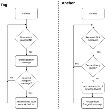
The system is able to automatically register when new devices are joining the network, and as such automatically hand out network addresses to all new devices. This is done by having the tag issue a broadcast message once a second, in order to allow any new non-registered devices to answer back, letting the tag know there is an additional device available. The broadcast message is what's called a Blink message, which is actually just a very short message containing no info.
* TODO: Write some more about this, and possibilities of auto-positioning for rapid-deployment
Ranging

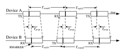
In order to estimate the distance between an anchor and a tag, the system uses Time of Flight (TOF). There exists a number of ways to estimate a distance from exchanging packages with timestamps, all with different pros and cons, which has been discussed elaborately in the DW1000 User manual. In this project, it has been chosen to implement and use the double-sided two way ranging scheme as shown in the figure to the right. This method has the advantage that it is the best method for handling any clock skew between the two devices, this means that it will have a smaller impact on the range estimate, if the clock in one device is running slightly faster than the clock of the other device.
The average time of flight between the two devices can be calculated as
From this the distance can be calculated by multiplying the propagation time with the speed of light.
The DS-TWR ranging scheme mentioned above can then be extended through the use of broadcast messages, in order to minimize the required number of data exchanges between devices. One such way could be through the infrastructure based asset tracking scheme as implemented in this project. In this ranging scheme the tag sends a Poll message as a broadcast, which is received by a number of anchors (three in the following case) in the infrastructure. Each anchor then replies in successive responses with packets RespA, RespB & RespC after which the tag, sends the Final message as a broadcast again, received by all three anchors. This allows the tag to be located after sending only 2 messages and receiving 3 (including another 3 if the distances are needed on the tag).
This scheme is illustrated in the figure below. This represents a substantial saving in message traffic, thereby saving battery power and air-time, while increasing potential update rate.
* TODO: Write a bit about peer-to-peer ranging schemes for lower update rate, but where every device knows the distance to every other device.
Positioning
The 3d position of the tag can be estimated, through multilateration by using ranges to at least four different anchors.
Because there is noise in the distance estimations performed by the system, the multilateration has the issue of becoming an optimization problem. This is because there is no exact solution to the multilateration problem at hand, but there will exist a solution that minimizes the sum of the errors in the euclidean distances. Mathematically speaking that is a position solution (x,y,z) that will minimize the term
Furthermore the complexity of the optimization tends to increase with more anchors being added into the system.
There are a few ways to solve the optimization problem described above, some of which will be discussed here.
Nonlinear least squares optimization
The direct way of solving the multilateration problem, would be through a least squares approximation. This is an iterative way of solving the problem in a purely non-statistical way, which means that it does not take into account what the previous solution was, and as such allows the tag to move an infinite distance between two consecutive samples. Another downside of the least squares method for solving the optimization problem, is that it is slightly harder to extend the system to provide more details, like velocity estimates.
Particle filter
Another way of solving the optimization problem, is by utilizing a statistical particle filter, also known as a sequential Monte Carlo filter. The base idea of a particle filter, is that a number of "particles", containing a direction and a speed, is spawned in a distributed manner and is then perturbed, with the goal of having the particles converge towards the same point, with a unified direction and speed.
The particle filter is a statistical filter, meaning that it takes into account the previous solutions found.
The particle filter has not been implemented or tested for this project, but a sample implementation, in Python, of such filter for this specific use case can be found at [https://github.com/bitcraze/lps-ros].
Extended Kalman filter
The last method of solving the optimization problem discussed here, will be the Extended Kalman filter. This way is, like the particle filter, a statistical filter.
Sensor fusion
TODO.
Limitations
The system does come with a few limitations, which will be discussed below.
Line of sight (LOS)
The most important limitation is that it is very sensitive to line of sight (LOS). This means that the tag trying to localize itself, should always have pure line of sight to at least 4 anchors, which is why it is recommended to run the system with 6 or more anchors, as this would give the system redundancy. It is possible to get a clue about whether the most recent range measurement was taken in a line of sight situation or not, by looking at the quality of the measurement. This quality is a combination of the received power level and the first path power level, and is discussed further in the DW1000 User manual on page 45.
Calibration
Because the system is based on time of flight measurements of radio waves, even a small change in the time stamps of the system will result in huge variations in distance (1 ns results in a change of 299 mm). This means that proper calibration of the system is crucial in order to obtain any usable performance. The main calibration property of the system is the antenna delay constants, a constant describing the delay from antenna through PCB. A detailed explanation of the antenna delay and how to calibrate it properly can be found in APS014: Antennna Delay Calibration
Range
The range of the system varies tremendously, as a function of channel, header length, data rate, transmission power etc. A longer communication range usually means a lower data rate and a less accurate distance estimate of the system. With the configuration currently chosen for the system, the range is about 25 m, as the system is configured for the best distance approximation as possible. The relatively short range is however not a problem in this case, as the system is intended to be used indoors, where a room is seldom larger than 25 meters end-to-end.
Received signal strength bias
TODO: What other limitations does the system come with?
Results to date
BIG TODO
Further work
- Multiple tags
- Relative positioning
- Peer-to-peer mesh ranging scheme
- Sensor fusion in EKF or preferably UKF
- Message push-through option
- Logging
Further reading
TODO: Add a link to decawaves resources page, talk about the google-groups group and mention the "Relevant papers" folder in Github

